packages <- c("tidyverse", "psych", "ggpubr", "ggcorrplot")
packages <- lapply(packages, FUN = function(x) {
if(!require(x, character.only = TRUE)) {install.packages(x)
library(x, character.only = TRUE)}})
data <- diamonds
class(data$price) # "integer"
class(data$carat) # "numeric"
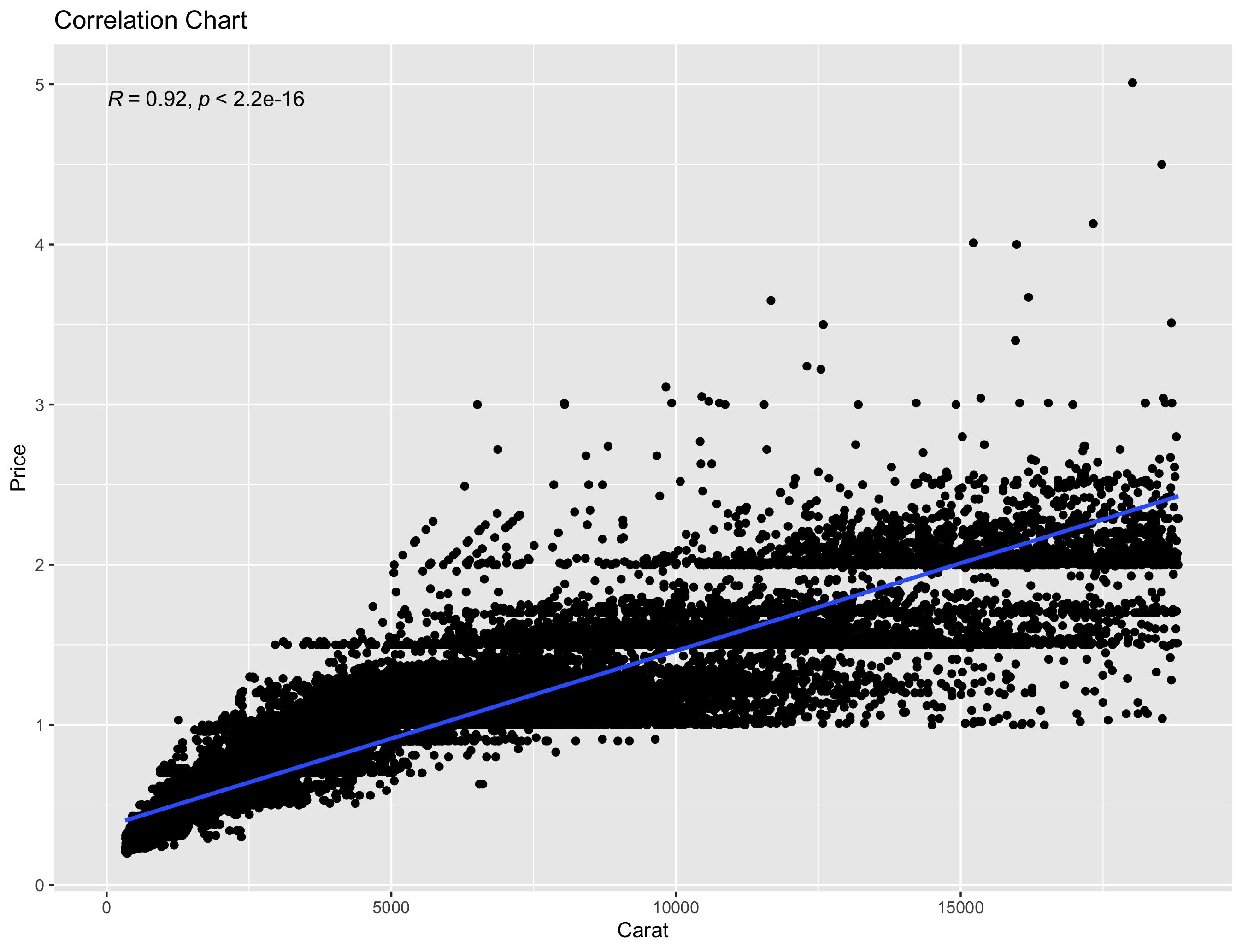
corr.test(data$price, data$carat)
correlation.plot <- ggplot(data, aes(price, carat)) +
geom_point() +
geom_smooth(method = lm) +
stat_cor(method = "pearson", label.x = 20) +
ggtitle("Correlation Chart") +
labs(y = "Price", x = "Carat")
correlation.plot
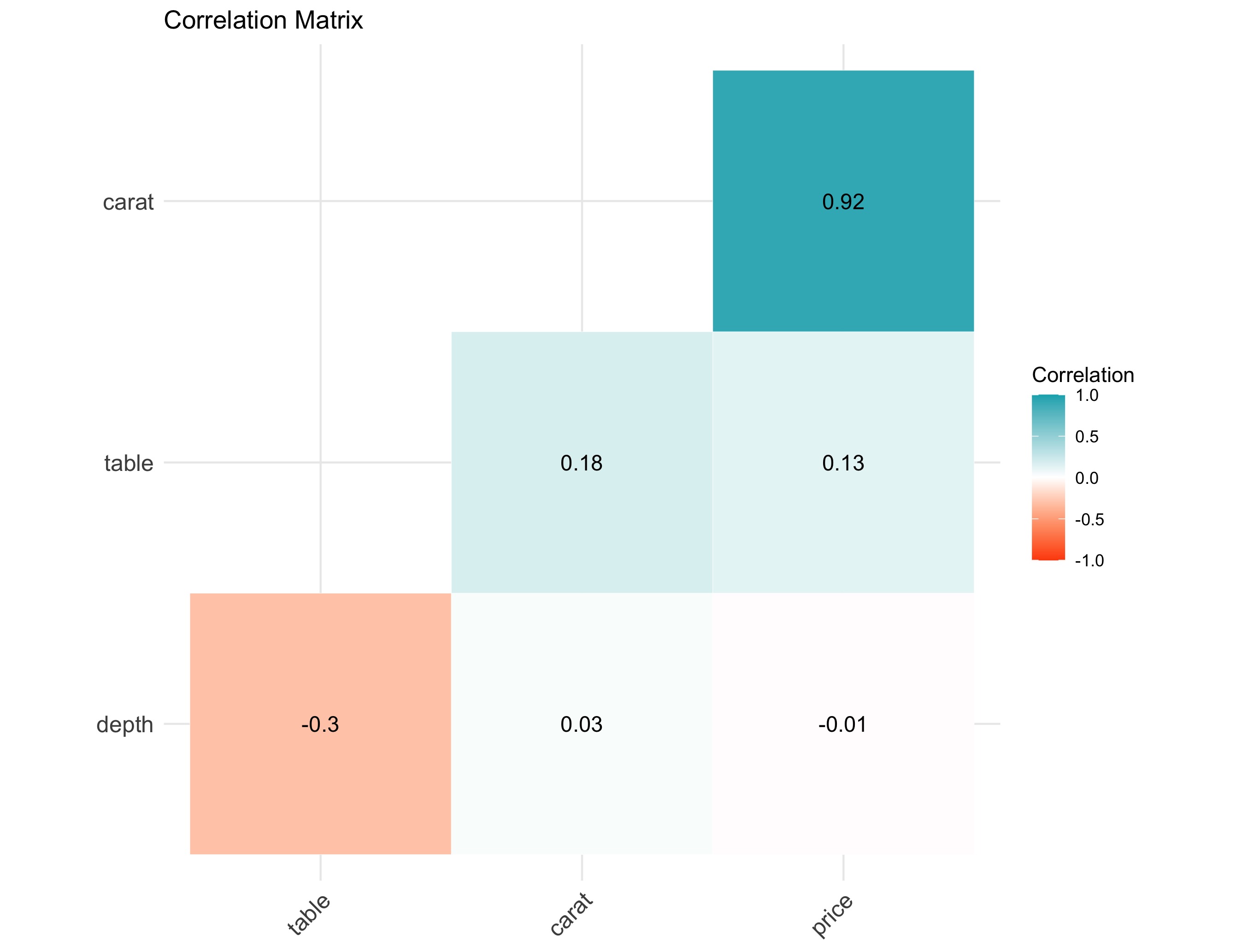
correlation.matrix <- dplyr::select(data, c(carat, depth, table, price))
correlation.matrix[correlation.matrix == ""] <- NA
correlation.matrix <- na.omit(correlation.matrix)
corr <- cor(correlation.matrix)
correlation.matrix.plot <- ggcorrplot(corr, p.mat = cor_pmat(correlation.matrix),
title="Correlation Matrix",
hc.order = TRUE, type = "lower",
color = c("#FC4E07", "white", "#00AFBB"),
outline.col = "white", lab = TRUE, legend.title = "Correlation")
correlation.matrix.plot
correlation.model <- cor.test(diamonds$price, diamonds$carat, method = c("pearson", "kendall", "spearman"))
correlation.model <- plyr::ldply (correlation.model, data.frame)
colnames(correlation.model)[1] <- "Attribute"
colnames(correlation.model)[2] <- "Value"
correlation.model <- correlation.model[-c(1,2,5,6,7,8,9,10), ]
correlation.model
correlation.table <- ggtexttable(correlation.model, rows = NULL, theme = ttheme("mBlue")) %>%
tab_add_title(text="Pearson's Correlation", face="bold", padding=unit(0.1, "line"))
correlation.table